
Orbital / IFS / Strange Attractor Properties Page
The Fractal Science Kit fractal generator Orbital / IFS / Strange Attractor page holds a set of properties specific to Orbital fractals and is visible only if the Fractal Type on the General page is set to Orbital / IFS / Strange Attractor.
See also:
The following pages are found in the page hierarchy under the Orbital / IFS / Strange Attractor page:
- Orbital Equation
- Transformation 1
- Symmetry Transformation
- Transformation 2
- Normalization
- Controllers
- Adaptive Smoothing
The Orbital Equation defines the fundamental equation used to compute the orbit points. As the orbit points are computed, statistics are added to the sample data that eventually will be used by the controllers to color the fractal. However, the orbit point is not added directly to the sample statistics. Rather, it is first passed to several programs that can transform the point prior to accumulating the statistics. Manipulating these programs can result in significantly different images, yielding countless variations for a given equation.
In the following discussion, let the orbit point generated by the orbital equation be called P. It is understood that even though the following discussion talks of transforming P, it is not meant to imply that these changes are included in the point passed to the orbital equation on the next iteration.
First, the orbit point P is transformed by Transformation 1. When a point P is transformed, it is understood that P is passed through the transformation and the resulting transformed point placed back in P.
Next P is passed to the Symmetry Transformation. A Symmetry Transformation takes a single input point P and transforms it into 0 or more points. Let the resulting set of N points be called P[N]. Each of the N points in P[N] is now passed to Transformation 2.
Any or all of these transformations can be set to the identity transformation, thereby skipping that step. In fact, it is usually the case that most (or all) of these transformations are the identity transformation. However, selective use of these transformations along with other Orbital fractal properties can result in highly unusual images.
Normalization controls the Data Normalization applied to the sample data. The Controllers page lets you set the list of Orbital Controllers used to process this fractal. Adaptive Smoothing is used to activate and control adaptive smoothing of the sample data.
Several of the properties on this page can be overridden in the Orbital Equation instructions using the FSK.OverrideValue method. See FSK Functions for details.
Orbital / IFS / Strange Attractor
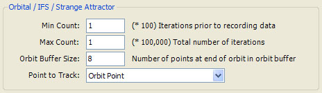
The Orbital / IFS / Strange Attractor section holds several properties associated with Orbital fractals. Orbital fractals process a single orbit with thousands (or millions) of iterations. Min Count (x 100) defines the number of iterations to process before collecting data. Max Count (x 100,000) defines the total number of iterations. Usually, you will set Max Count to a small number and increase it when you find an interesting fractal whose image you want to save. Max Count is rarely set to a value larger than 200. In truth, the total number of iterations is also adjusted for any oversampling associated with Anti-Aliasing and for the size of the image so the actual number of iterations is:
Iterations = MaxCount * 100000 * SamplesPerPixel * ImageSizeFactor
SamplesPerPixel in the above equation is 1 if Oversampling is <None>, 4 for 2x2 Oversampling, 9 for 3x3 Oversampling, and 16 for 4x4 Oversampling. For example, if Max Count is 50 and Oversampling is set to 2x2 Oversampling, the number of iterations is 20,000,000 (assuming ImageSizeFactor is 1).
ImageSizeFactor is derived from the size of the image relative to the default size of 600 by 450. For example, if you increase the image size to 1200 by 900, the ImageSizeFactor would be 4 since there are 4 times as many pixels in the image. Adjusting the number of iterations based on ImageSizeFactor lets you change the image size without having to adjust the Max Count to get the same image quality.
Since Orbital fractals do not generate an orbit per sample as do Mandelbrot fractals, Anti-Aliasing does not result in as severe a time penalty as with Mandelbrot fractals, and it is recommended that you set Oversampling to one of the higher settings when exploring Orbital fractals since the increased quality outweighs the cost.
Clearly, keeping track of all the orbit points is not feasible given these large numbers, so a small buffer of orbit points is maintained throughout the iteration which contains the last Orbit Buffer Size points. This determines the number of points available to your programs via the Orbit Functions. The default Orbit Buffer Size is 8 and is rarely changed.
During the iteration, the orbit points are examined and the orbit is terminated early if the orbit diverges or the orbit point becomes NaN (Not a Number) usually indicating an error condition or an undefined operation was performed (e.g., 0/0). If the orbit terminates early, the reason it did so will be given in the Information Window.
For each point that we visit during the orbit, we accumulate statistics in the associated sample point. These statistics are made available to the controllers to use when mapping the samples to colors. Normally, we track the orbit point as it moves from point to point, but this can be changed using the Point to Track property. The possible settings are:
- Orbit Point
- Orbit Transformation Point
- Triangle Metric Point
The default, Orbit Point, simply tracks the orbit point. Orbit Transformation Point and Triangle Metric Point track the points defined by the Orbit Transformation and Triangle Metric Pages. For example, if Point to Track is set to Triangle Metric Point and the Triangle Metric is set to the CircumCenter of the last 3 orbit points, instead of visiting each orbit point, we find the CircumCenter for the last 3 orbit points and visit that point instead.