
Classic Controllers Overview
Classic Controllers are programs (called controllers hereafter) used by the Fractal Science Kit fractal generator to map sample data collected during the fractal iteration, to colors for display. Each controller is composed of a set of properties and instructions. The properties are in a set of sections at the top of the page and the instructions are at the bottom of the page. To view the instructions, use the editor's Toggle Code View button to hide the properties and expand the instructions to fill the space.
As the sample points are processed by the Fractal Science Kit fractal generator, each sample is passed to the (single) Classic Master Controller who calls 0 or more Classic Controllers to process the sample. The controller's instructions are responsible for assigning a Color to the special variable color based on selected fields in the sample. The properties include a set of gradients and/or textures that can be accessed within your instructions, as required. You can use sample data to select which gradient/texture to reference, and to index into the selected gradient/texture to obtain a color. Alternatively, you can use sample data to create a color directly.
After the color is returned from your instructions, the controller uses the property settings on this page to further process the color as defined below.
See also:
- Mandelbrot Fractal Overview
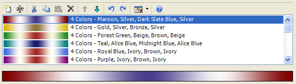
- Gradient List Control
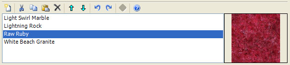
- Texture List Control
- Color Controllers
- Controllers
- Properties Window
- Program Editors
- Fractal Programs
- Program Instructions
- Programming Language
Each program is composed of a set of properties and instructions.
Comments
Always remember to click the Toggle Code View toolbar button at the top of the Program Editor and read the comments given in the comment section of the program's instructions. The comment section contains usage instructions, hints, notes, documentation, and other important information that will help you understand how best to use the program. Once you are done reading the comments, click the Toggle Code View toolbar button again to view the program's properties.
Gradients
The following properties are defined in the Gradients section:
-
Gradients are the ordered list of gradients available to the controller. The Gradient List Control allows you to add/remove gradients to/from the list, reorder the list, cut/copy/paste gradients between lists on other properties pages, undo/redo list changes, edit gradients in the list using the Gradient Editor, and open the Gradient Browser so you can copy/paste existing gradients from the Built-in Gradients or My Gradients into the list. When you paste a gradient into the list, a copy of the gradient is made so that any changes to the gradient will not affect the original. Your program can access this list using the Gradient Functions.
Textures
The following properties are defined in the Textures section:
-
Textures are the ordered list of textures available to the controller. The Texture List Control allows you to add/remove textures to/from the list, reorder the list, cut/copy/paste textures between lists on other properties pages, undo/redo list changes, and repair broken textures. Your program can access the list using the Texture Functions. Each texture in the list is displayed using the name of the associated texture file without the file extension. If a single texture is selected, the texture's image is displayed in the preview area on the right side of the control. If the texture file no longer exists or cannot be loaded, the name will also include the text [error loading file] and a default texture (a white box) is used. You should replace these items or remove them from the list. To replace a broken texture in the list, simply select it and click the Repair toolbar button and select the replacement.
Properties
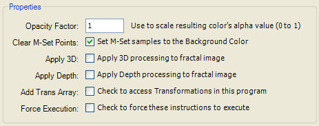
The following properties are defined in the Properties section:
-
Opacity Factor is used to scale the resulting color's Alpha value. The Alpha value is an indication of the color's opacity. The Alpha value ranges from 0 to 1, where 0 is transparent and 1 is fully opaque. The Opacity Factor can be used to scale the Alpha value of each color produced by this controller.
-
Clear M-Set Points is used to automatically return a transparent color (i.e., a color whose Alpha is set to 0) for samples that are inside (part of) the Mandelbrot set. That is, for Divergent fractals, a transparent color is used for samples whose orbit did not escape; i.e., the orbit point did not exceed the Bailout value when the maximum number of iterations (Max Dwell) was reached. For Convergent fractals, a transparent color is used for samples whose orbit did not converge; i.e., the distance between 2 consecutive orbit points did not fall below Epsilon when the maximum number of iterations (Max Dwell) was reached. Uncheck Clear M-Set Points to handle the mapping of these samples within the program. Check Clear M-Set Points to map samples determined to be part of the Mandelbrot set to a transparent color (your program is never called). If you uncheck Clear M-Set Points, you should turn off Cycle Detection since this tends to alter the statistics associated with inside samples. The values Bailout, Epsilon, and Max Dwell, are defined in the Orbit Generation section of the Mandelbrot / Julia / Newton page.
-
Apply 3D is used to turn on 3D processing and enable the 3D Mapping properties (described below). 3D processing uses the value of one of the sample fields to obtain a virtual height, and scales the color based on this height in conjunction with the 3D Mapping properties.
-
Apply Depth is used to turn on depth processing and enable the Depth Mapping properties (described below). Depth processing uses the value of one of the sample fields to obtain a virtual depth, and darkens/lightens the color based on this depth in conjunction with the Depth Mapping properties.
-
Add Trans Array is a checkbox that can be checked to add a Transformation Array editor as one of the program's properties pages. Users can add 1 or more transformations to the editor and your program can access the transformations using the Transformation Functions.
-
Force Execution is a checkbox that can be checked to force execution of the instructions. If Force Execution is unchecked, the instructions will execute only if required based on what changes were made to the fractal's properties since the last time the instructions ran. This is rarely checked.
Color Space Adjustment
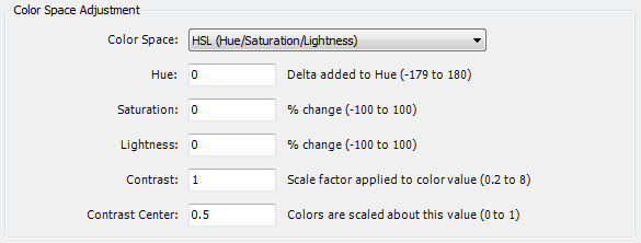
The Color Space Adjustment section is used to adjust individual components of the HSL (Hue/Saturation/Lightness) or HSV (Hue/Saturation/Value) color space. The adjustments are applied to the color returned by your program.
To use these settings, you select the color space you want to adjust (HSL or HSV) and then set the values for the individual components associated with the selected color space. The HSL color model supports Hue, Saturation, and Lightness components. The HSV color model supports Hue, Saturation, and Value components. The Hue is identical in both color models but the Saturation is quite different. The Lightness and Value components are unique to the HSL and HSV color models, respectively.
See HSL and HSV for details on these color models.
The following properties are defined in the Color Space Adjustment section.
-
Color Space is the color space you want to adjust. It can be set to HSL (Hue/Saturation/Lightness) or HSV (Hue/Saturation/Value). The HSL color space supports adjustments to the Hue, Saturation, and Lightness of the color. The HSV color space supports adjustments to the Hue, Saturation, and Value of the color.
-
Hue is a value added to the color's Hue. The value should be between -179 and 180.
-
Saturation is a value between -100 and 100 used to scale the color's Saturation. The value is given as a percentage change relative to the color's current Saturation. For example, 25 would increase the color's Saturation by 25 percent of the difference between full saturation and the current value. A value of -40 would reduce the color's Saturation by 40 percent.
-
Lightness is a value between -100 and 100 used to scale the color's Lightness. The value is given as a percentage change relative to the color's current Lightness. Lightness is unique to the HSL color model.
-
Value is a value between -100 and 100 used to scale the color's Value. The value is given as a percentage change relative to the color's current Value. Value is unique to the HSV color model.
-
Contrast is a value between 0.2 and 8 used to scale the color's Lightness/Value about the central value (Contrast Center). Values greater than 1 increase contrast. Values less than 1 decrease contrast. Lightness is used for the HSL color model. Value is used for the HSV color model.
-
Contrast Center is the central value about which Contrast scaling is applied.
Color Adjustment
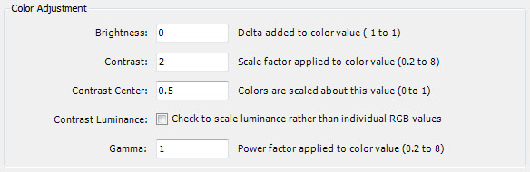
The Color Adjustment section is used to adjust the brightness, contrast, and gamma of the color returned by your program.
The following properties are defined in the Color Adjustment section.
-
Brightness is a value added to each color's RGB components. The value should be between -1 and 1. Positive values brighten the color, negative values darken the color.
-
Contrast is a value between 0.2 and 8 used to scale each RGB component of the image data about the central value (Contrast Center). Values greater than 1 increase contrast. Values less than 1 decrease contrast.
-
Contrast Center is the central value about which Contrast scaling is applied.
-
Contrast Luminance is a Boolean that, when checked, scales the color's luminance rather than individual RGB values when applying contrast.
-
Gamma is a power factor applied individually to each color's RGB components. The value should be between 0.2 and 8. Values greater than 1 brighten the color. Values less than 1 darken the color.
3D Mapping
The 3D Mapping section applies 3D shading to the color returned by your program. A data value is mapped to a virtual height and a simple 3D shading model is applied to the image. Properties are provided to control the light intensity, ambient light, and specular reflection. Additional properties control the data/height mapping.
The 3D Mapping processing supports 2 different lighting models. The first lighting model maps a sample field to a height and assumes a single light source directly above the surface. The second lighting model uses a surface normal vector and 1 or 2 light sources to determine the amount of light that is displayed at a given point. To use the second lighting model, you set the Map To property to Surface Normal or Surface Normal (Restricted).
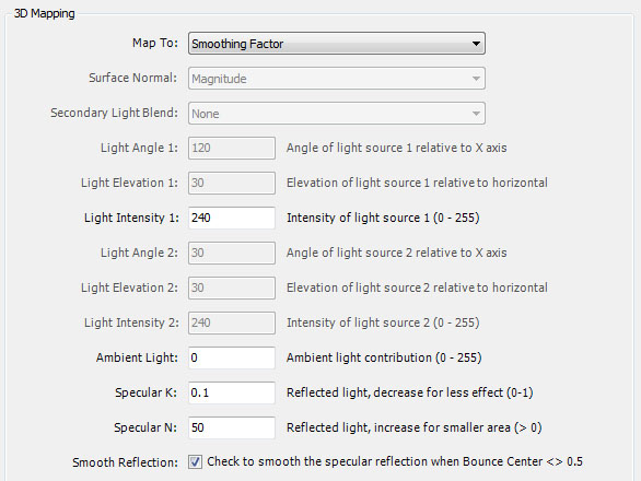
Map To is the data value mapped to height when performing 3D processing.
If you set Map To to one of the sample fields or Composite Height, the lighting model assumes a single light source directly above the surface. Set Map To to Composite Height to access the value of compositeHeight, computed by your instructions. It is expected that compositeHeight is set to a value between 0 and 1. By default, a value of 0 maps to a visual high and a value of 1 maps to a visual low.
Set Map To to Surface Normal or Surface Normal (Restricted) to use a surface normal vector and 1 or 2 light sources to determine the amount of light that is displayed at a given point. The surface normal settings enable the Surface Normal property (see below) to specify what surface normal vector should be used for processing. The Surface Normal (Restricted) setting is quick to set up but has far less flexibility than the unrestricted version and many of the 3D Mapping properties are disabled. When using the restricted version, you will probably need to add some ambient light or use 2 light sources to get the best results.
When you set Map To, the properties appropriate for the associated lighting model are enabled, and the properties not appropriate for the associated lighting model are disabled.
The Surface Normal property determines which surface normal vector to use. Surface Normal can be set to Magnitude, Alternate 1 Value, Alternate 2 Value, or Trap Value. Of course, in order to use Alternate 1 Value or Alternate 2 Value, you will need to define an Alternate Mapping for Alternate Mapping 1 or Alternate Mapping 2. Similarly, in order to use Trap Value, you will need to set the Type property on the Mandelbrot / Julia / Newton page to Both and set Process Orbit Trap to Generate Data and set up an Orbit Trap.
See the following pages for additional control over the surface normal computation related to these data values:
Secondary Light Blend is used to define a second light source for the surface normal lighting model, and to set the blending function used to blend the 2 light sources together. There are quite a few blending functions, and you can experiment with the different settings to see which one produces the best results in a given situation. If Secondary Light Blend is None, a single light source is used.
Light Angle 1, Light Elevation 1, and Light Intensity 1, define the angle, elevation, and intensity of the first light source. Light Angle 2, Light Elevation 2, and Light Intensity 2, define the angle, elevation, and intensity of the second light source. The light angle is given as an angle (in degrees between -360 to 360) relative to the X axis. The light elevation is given as an angle (in degrees between -360 to 360) relative to horizontal. Normally, the elevation is between -60 and 60 but this is not required. The light intensity is an integer between 0 and 255 that represents the intensity of the light source. A value of 0 is void of light and a value of 255 is full intensity. This value is normally between 200 and 240.
Ambient Light is an integer between 0 and 255 that represents light that reaches the object reflected off other objects. A value of 0 includes no ambient light. This value is normally between 0 and 20.
Specular K is a value between 0 and 1 that represents a specular reflection constant. This value is normally between 0.01 and 0.1 where smaller values result in less specular reflection. This property is disabled for the surface normal lighting model and you should check Apply Highlight below to add highlights to the image.
Specular N is an integer greater than 0 that represents a specular reflection exponent. This value is normally between 5 and 100. Use small values for larger, less intense highlights, large values for smaller, more intense highlights. This property is disabled for the surface normal lighting model and you should check Apply Highlight below to add highlights to the image.
Smooth Reflection is a Boolean that, when checked, applies a smoothing function to the specular reflection. This property is disabled for the surface normal lighting model.
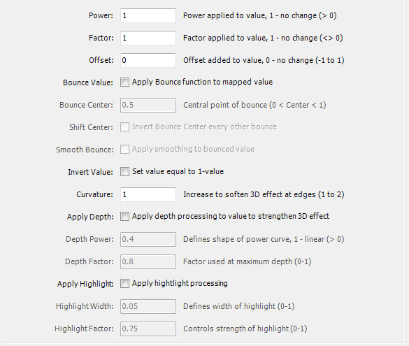
The remainder of the 3D Mapping section contains properties to adjust the data mapping.
Power, Factor, and Offset are applied to the value.
value ^= Power
value *= Factor
value += Offset
When using the surface normal light model, Factor is normally between 0.5 and 2 (or -0.5 and -2) but can fall outside that range on occasion.
The Power, Factor, and Offset adjustments, can result in values outside the range 0 to 1. Each value is mapped to a unit index and wrapped into the range 0 to 1.
Bounce Value is a Boolean value that, when checked, applies the Bounce function to the value before using it. This results in the heights moving up and down in a zigzag pattern (triangle wave). If Bounce Value is False (unchecked), the heights ramp up or down in a sawtooth pattern. This property is checked and disabled for the surface normal lighting model.
Bounce Center is a value between 0 and 1 that is used to adjust the peak when Bounce Value is checked. Normally this value is 0.5 to place the peak in the center of the band. Values like 0.25 and 0.75 move the peak to the inside/outside of the band and are nice variations. Bounce Center is disabled if Bounce Value is unchecked.
Shift Center is a Boolean value that, when checked, inverts the Bounce Center every other unit. Shift Center is disabled if Bounce Value is unchecked.
Smooth Bounce is a Boolean value that, when checked, applies a smoothing function to the bounced value resulting in a sine wave rather than a triangle wave. Smooth Bounce is disabled if Bounce Value is unchecked.
Invert Value is a Boolean value that, when checked, replaces value with 1-value. Highs become lows and lows become highs.
Curvature is used to soften the 3D effect. A value of 1 is maximum curvature and results in the strongest 3D effect. Values greater than 1 increase the radius of curvature and soften the 3D effect.
Apply Depth is a Boolean value that, when checked, strengthens the 3D effect by adding depth to the value. In some cases this adds a metallic quality to the resulting colors.
Depth Power defines the shape of the power curve used for depth processing.
Depth Factor is the factor applied to the value at maximum depth.
Apply Highlight is a Boolean value that, when checked, adds highlights to the image. Normally, you should check Apply Highlight when using the surface normal lighting model, but you can check Apply Highlight to strengthen the highlights even when not using the surface normal lighting model.
Highlight Width controls the width of the highlight.
Highlight Factor controls the strength of the highlight.
Depth Mapping
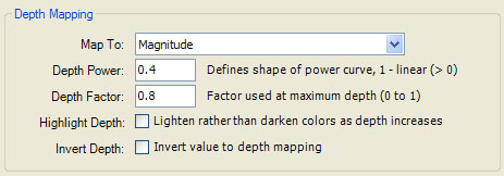
The Depth Mapping section applies depth shading to the color returned by your program. One of the sample data fields is mapped to a virtual depth and a simple depth shading model is applied to the image. Properties are provided to control the power/factor used to define the sample/depth mapping, and to lighten rather than darken the colors as the depth increases.
The following properties are defined in the Depth Mapping section.
-
Map To is the sample field mapped to depth when performing depth processing. In addition to the sample fields, you can set Map To to Composite Depth to access the value of compositeDepth, computed by your instructions. It is expected that compositeDepth is set to a value between 0 and 1.
-
Depth Power defines the shape of the power curve used for depth processing.
-
Depth Factor is the amount of black (or white if highlighting) that is blended into a color at maximum depth.
-
Highlight Depth is a Boolean value that, when checked, lightens rather than darkens the color based on depth.
-
Invert Depth is a Boolean value that, when checked, replaces depth with 1-depth.
Instructions
The remainder of this page can be ignored if you are not a programmer.
At the bottom of the window is an editor pane named Instructions. The editor pane is a simple text editor to view/edit your Program Instructions. See Editing Text for details.
The instructions are divided into sections. Within each section are statements that conform to the Programming Language syntax.
In addition to the Standard Sections, Classic Controllers support 1 other section:
color:
This section is responsible for setting the color for the current sample point. The color is returned in the built-in variable color.
Built-in Variables
Several built-in variables are available to your instructions:
- Color color
- compositeHeight
- compositeDepth
- pixel
Controllers can access the above built-in variables. color is used to return the color computed by the program.
compositeHeight is used to return a value for the Map To setting in the 3D Mapping section. That is, if the 3D Mapping section's Map To is set to Composite Height, the instructions should set compositeHeight to a value between 0 and 1 for this purpose. Otherwise, compositeHeight need not be set. compositeHeight is rarely used.
compositeDepth is used to return a value for the Map To setting in the Depth Mapping section. That is, if the Depth Mapping section's Map To is set to Composite Depth, the instructions should set compositeDepth to a value between 0 and 1 for this purpose. Otherwise, compositeDepth need not be set. compositeDepth is rarely used.
pixel is the location in the complex plane of the current sample point and is read-only.
color is a Color object defined as:
Object Color {
R|Red |H|Hue
G|Green|S|Saturation
B|Blue |L|Lightness |V|Value
A|Alpha
}
Each of the fields should be a floating point value between 0 and 1, inclusive. See the Color Functions for details.
The Color object supports the RGB, HSL, and HSV color models but the Fractal Science Kit expects color to conform to the RGB color model. If your program generates a color using the HSL or HSV color model, you must convert the color to the RGB color model prior to returning.
The color's Alpha value is used to set the color's opacity. A value of 0 makes the color totally transparent and a value of 1 makes the color totally opaque. Values between 0 and 1 can be used to define colors that are translucent. The controller's Opacity Factor is applied to color's Alpha value set by the instructions.
Example:
color:
color = Gradient.Color(0, Sample.Magnitude)
This example calls the Gradient Function Gradient.Color to map the sample's normalized magnitude (Sample.Magnitude) to a color using the 1st gradient in the controller's list of gradients (i.e., gradient 0).
Another common method of accessing the sample data is to use a SamplePointValue Option to allow the user to select a field from the Sample object (described below) using the associated property on the Properties Page.
Example:
color:
color = Gradient.Color(0, Value)
properties:
option Value {
type = SamplePointValue
caption = "Value"
default = Sample.Magnitude
}
This example maps a user selected SamplePointValue called Value, to a gradient index thereby obtaining a color. Unlike other option types, a SamplePointValue option does not return a constant, but instead, uses the SamplePointValue setting to access the corresponding component of the current sample which is returned by the option (in this case, Value). In this example, the option's default value is given as Sample.Magnitude which equates to the previous example if the user does not change it.
Example:
comment:
Maps a sample point value to a gradient index.
color:
color = Gradient.Color(ColorScheme, Value)
properties:
option ColorScheme {
type = GradientIndex
caption = "Color Scheme"
default = 0
size = Large
}
option Value {
type = SamplePointValue
caption = "Value"
default = Sample.Magnitude
}
Like the previous example, this controller maps a user selected SamplePointValue to a gradient index thereby obtaining a color. However, instead of simply using controller 0 as in the previous example, this controller calls the function Gradient.Color(ColorScheme,Value) to map the sample data to a color using the gradient in the controller's list of gradients indexed by ColorScheme. See GradientIndex Options for details.
Example:
color:
color = Gradient.Color( \
Offset2 + Factor2*Value2^Power2, \
Offset1 + Factor1*Value1^Power1 \
)
properties:
divider {
caption = "Value"
}
option Value1 {
type = SamplePointValue
caption = "Value"
default = Sample.Magnitude
}
option Power1 {
type = Float
caption = "Power"
details = "Set value = value ^ Power (0.125 to 8)"
default = 1
range = [0.125,8]
}
option Factor1 {
type = Float
caption = "Factor"
details = "Set value = value * Factor (-8 to 8)"
default = 1
range = [-8,8]
}
option Offset1 {
type = Float
caption = "Offset"
details = "Set value = value + Offset (-1 to 1)"
default = 0
range = [-32,32]
}
divider {
caption = "Overlay"
}
option Value2 {
type = SamplePointValue
caption = "Overlay"
default = Sample.Alternate1Value
}
option Power2 {
type = Float
caption = "Power"
details = "Set overlay = overlay ^ Power (0.125 to 8)"
default = 1
range = [0.125,8]
}
option Factor2 {
type = Float
caption = "Factor"
details = "Set overlay = overlay * Factor (0 to 32)"
default = 8
range = (0,32]
}
option Offset2 {
type = Float
caption = "Offset"
details = "Set overlay = overlay + Offset (-1 to 1)"
default = 0
range = [-1,1]
}
This example uses 2 SamplePointValue options (Value1 and Value2) to superimpose 1 design on top of another. The color section is the single statement:
color = Gradient.Color( \
Offset2 + Factor2*Value2^Power2, \
Offset1 + Factor1*Value1^Power1 \
)
As in the previous examples, we call the function Gradient.Color to map the sample to a color, but here we use Value2 to select 1 of the 2 gradients in the controller's list, and use Value1 to index into the selected gradient to obtain a color. Gradient.Color wraps both arguments at the extremes. The 1st argument is an integer index into the list of gradients. If the list contains 2 gradients as in this example, even values map to the 1st gradient and odd values map to the 2nd gradient. The argument is truncated to an integer before use. The 2nd argument to Gradient.Color is a real number between 0 and 1. Values outside this range are wrapped before selecting the color. For example, passing 1.2 would return the color at position 0.2.
Example:
color:
color = Color(R, G, B, 1)
properties:
option R {
type = SamplePointValue
caption = "R"
default = Sample.Magnitude
}
option G {
type = SamplePointValue
caption = "G"
default = Sample.Alternate1Value
}
option B {
type = SamplePointValue
caption = "B"
default = Sample.Alternate2Value
}
This example maps 3 SamplePointValue options directly to the RGB components for Red, Green, and Blue.
Constants
The following constants are available to your instructions:
- ViewportMagnification
- MinimumDwell
- MaximumDwell
ViewportMagnification is the current fractal's magnification. The magnification can be viewed by executing the Resize command on the View menu of the Fractal Window. MinimumDwell and MaximumDwell give the range of dwells in the image and are only available in the color: section of the program.
Accessing Sample Data
The data associated with the sample being processed is accessed by the controller using the Sample object. The Sample object is a read-only object that contains all the collected data for the sample point. Many of the fields have been normalized based on normalization settings for the associated field, and the value is between 0 and 1. In some cases both the raw value and the normalized value are available.
The following fields are associated with the Sample object for Classic Controller programs:
- Sample.IsInside
- Sample.Dwell
- Sample.DwellRaw
- Sample.Angle
- Sample.AngleBounce
- Sample.AngleCos
- Sample.AngleRaw
- Sample.SmoothAngle(power)
- Sample.SmoothAngleBounce(power)
- Sample.SmoothAngleCos(power)
- Sample.SmoothAngleRaw(power)
- Sample.Magnitude
- Sample.RootIndex
- Sample.RootIndexRaw
- Sample.SmoothingFactor
- Sample.Alternate1Value
- Sample.Alternate1ValueRaw
- Sample.Alternate1Angle
- Sample.Alternate1AngleBounce
- Sample.Alternate1AngleCos
- Sample.Alternate1AngleRaw
- Sample.Alternate1Index
- Sample.Alternate1IndexRaw
- Sample.Alternate2Value
- Sample.Alternate2ValueRaw
- Sample.Alternate2Angle
- Sample.Alternate2AngleBounce
- Sample.Alternate2AngleCos
- Sample.Alternate2AngleRaw
- Sample.Alternate2Index
- Sample.Alternate2IndexRaw
- Sample.IsTrapped
- Sample.TrapValue
- Sample.TrapAngle
- Sample.TrapAngleBounce
- Sample.TrapAngleCos
- Sample.TrapAngleRaw
- Sample.TrapDwell
- Sample.TrapDwellRaw
- Sample.TrapIndex
- Sample.TrapIndexRaw
- Sample.TrapDelta
- Sample.TrapDeltaRaw
- Sample.TrapCount
- Sample.TrapCountRaw
- Sample.TrapId
In the discussion below, the properties Bailout, Epsilon, Min Dwell, Max Dwell, Angle Reference Point, Magnitude, Reference Point, and Cos Smoothing, are defined in the Orbit Generation section of the Mandelbrot / Julia / Newton page.
Mandelbrot samples can be categorized by whether or not the associated orbit diverged (or converged if the fractal type is Convergent). If the orbit diverged (or converged), the sample is said to be outside the Mandelbrot set. Otherwise, it is said to be inside the set. Sample.IsInside is true if the sample is inside the Mandelbrot set, and false otherwise. That is, for Divergent fractals, Sample.IsInside is true for samples whose orbit did not escape; i.e., the orbit point did not exceed the Bailout value when the maximum number of iterations (Max Dwell) was reached. For Convergent fractals, Sample.IsInside is true for samples whose orbit did not converge; i.e., the distance between 2 consecutive orbit points did not fall below Epsilon when the maximum number of iterations (Max Dwell) was reached.
If the sample is outside the Mandelbrot set, Sample.DwellRaw is the dwell value at the end of the fractal iteration and ranges from Min Dwell to Max Dwell. If the sample is inside the Mandelbrot set, Sample.DwellRaw is Max Dwell + 1. I use Max Dwell + 1 rather than Max Dwell to differentiate the case where the point with dwell equal to Max Dwell is outside the Mandelbrot set. Sample.Dwell is the normalized dwell value. The normalized value is between 0 and 1.
Sample.AngleRaw is the angle (in radians) between the X axis and a line from the Angle Reference Point to the sample's last orbit point. All of the other angle values are normalized to the range 0 to 1. Sample.Angle is a straight linear mapping of the angle where 0 to 360 maps to 0 to 1. Sample.AngleBounce maps angles from 0 to 180 into values from 0 to 1, and maps angles from 180 to 360 into values from 1 to 0. That is, as the angle increases from 0 to 360, Sample.AngleBounce starts at 0, increases to 1 at the half-way point (180), and then decreases (bounces) back to 0. Sample.AngleCos is identical to Sample.AngleBounce except that it uses a cosine based wave rather than a triangle based wave so it is smoother at the extremes. Sample.SmoothAngle, Sample.SmoothAngleBounce, Sample.SmoothAngleCos, and Sample.SmoothAngleRaw are the smoothed angle versions of these functions. power must be greater than or equal to 1 and these functions are only valid for points outside the Mandelbrot set. power=1 is linear smoothing and smoothing increases with power.
The interpretation of Sample.Magnitude depends on the settings Magnitude, Reference Point, and Cos Smoothing and whether the point is inside or outside the Mandelbrot set.
If the point is inside the Mandelbrot set, Sample.Magnitude is the normalized magnitude of the sample's last orbit point. Sample.Magnitude ranges smoothly from 0 to 1 as the point's unnormalized magnitude ranges from 0 to Bailout (or 0 to Epsilon for Convergent fractals).
If the point is outside the Mandelbrot set, Sample.Magnitude is the normalized magnitude of the sample's last orbit point combined with the sample's dwell value such that a continuous value is generated across dwell boundaries. Sample.Magnitude ranges smoothly from 0 to 1 as the dwell increases from Min Dwell to Max Dwell. The Sample.Magnitude for all points with dwell N is less than that for those points with dwell N+1.
Sample.Magnitude normalization is based on the Classic properties page settings.
If Root Detection is active and you are generating a Julia fractal, the Fractal Science Kit will attempt to identify roots based on the Root Detection properties Epsilon, Threshold, and Max Roots. Root Detection is normally used for Convergent fractals (e.g., Newton fractals), but it can be used to color the samples inside the Mandelbrot set for Divergent fractals too. In that case, the roots represent points of convergence among those points that did not escape. Remember that you will need to uncheck the Clear M-Set Points checkbox and turn off Cycle Detection to color the samples inside the Mandelbrot set.
You can access the index of the root to which the sample converged, using the values Sample.RootIndexRaw or Sample.RootIndex. Sample.RootIndexRaw is a value from -1 to 1 less than the number of roots. Samples that converge to one of the roots have a value greater than or equal to 0. Samples that failed to converge to a root have the value -1. Sample.RootIndex is the normalized index and ranges from 0 to 1. Sample.RootIndex=0 for samples that failed to converge to a root.
Example:
comment:
This controller is intended for Newton fractals.
Newton Mandelbrots are displayed in a single color
but when you explore Julia fractals, they are in
full color.
Root Detection must be active to use this controller.
color:
color = Gradient.Color(0, Sample.RootIndex)
Root Detection is not applicable for Mandelbrot fractals; Sample.RootIndex and Sample.RootIndexRaw are 0 and -1, respectively, for all samples. However, a common approach is to activate Root Detection and use a controller like the one given above (e.g., Gradient Map - Newton) for the Mandelbrot fractal. Then use the Preview Julia feature to explore different Julia fractals by clicking on the Mandelbrot to define the Julia Constant for the preview. The Mandelbrot will be displayed using shades of a single color since Sample.RootIndex is 0 for all samples (the shading is due to 3D processing) but the Julia Preview will be rendered in full color based on the roots found during Root Detection.
Sample.SmoothingFactor is a smoothing factor associated with Continuous Potential Smoothing. It is a value that ranges from 0 to 1. If you consider only those samples associated with a given dwell value in a small region of the complex plane, samples with a smoothing factor close to 0 are farthest from the Mandelbrot set and samples with a smoothing factor close to 1 are closest to the Mandelbrot set. In practice, the smoothing factor is used to calculate the (un-normalized) magnitude as:
magnitude = dwell - 1 + Sample.SmoothingFactor
The Sample.SmoothingFactor is commonly used to smooth values across dwells.
The alternate value fields (Sample.Alternate...) are associated with data initialized on the Alternate Mapping pages. The fields named Sample.Alternate1... are associated with the data for Alternate Mapping 1 and the fields named Sample.Alternate2... are associated with the data for Alternate Mapping 2. If the type of either mapping is <None>, the associated sample fields are not initialized. Otherwise, the fields are initialized from the sample's AlternatePointInfo data given by the mapping. Recall that the AlternatePointInfo object is defined as:
Object AlternatePointInfo {
Value
Angle
Index
}
For example, consider the sample fields associated with Alternate Mapping 1.
Sample.Alternate1Value is the normalized Value and Sample.Alternate1ValueRaw is the raw (un-normalized) Value.
Sample.Alternate1AngleRaw is the raw radian Angle. All of the other angle values are normalized to the range 0 to 1. Sample.Alternate1Angle is a straight linear mapping of the angle where 0 to 360 maps to 0 to 1. Sample.Alternate1AngleBounce maps angles from 0 to 180 into values from 0 to 1, and maps angles from 180 to 360 into values from 1 to 0. That is, as the angle increases from 0 to 360, Sample.Alternate1AngleBounce starts at 0, increases to 1 at the half-way point (180), and then decreases (bounces) back to 0. Sample.Alternate1AngleCos is identical to Sample.Alternate1AngleBounce except that it uses a cosine based wave rather than a triangle based wave so it is smoother at the extremes.
Sample.Alternate1Index is the normalized Index and Sample.Alternate1IndexRaw is the raw Index.
The sample fields associated with Alternate Mapping 2 are defined similarly. If orbit trap processing is enabled, the sample fields associated with Alternate Mapping 2 are used to hold orbit trap related data and should not be used directly but rather, you should use the orbit trap fields as described below.
Mandelbrot processing can include both classic processing and orbit trap processing. If both are enabled, the sample data related to orbit traps can be used along with the classic data to map the sample to a color. Normally, you would use the Orbit Trap Controllers to process the samples that are trapped but this is not required. If you generate both Classic and Orbit Trap data but you set the Process Orbit Trap property on the Mandelbrot / Julia / Newton page to Generate Data rather than Activate Controllers, the orbit trap data will be generated but the Classic Controllers are called to process the trapped points rather than calling the Orbit Trap Controllers as is usually the case.
If orbit trap processing is enabled, Sample.IsTrapped is true if the point was trapped and false otherwise. Each of the other trap related fields (Sample.Trap...) are as described in Orbit Trap Controllers.